Accessibility data refers to the ease of reaching services and areas within a given timeframe using various transportation modes. This data, collected through modern tools and sensors, is vital for modern urban planning and property assessment. In this tutorial, we’ll focus on visualizing accessibility in Helsinki, particularly the time to access key services within a 30-minute walking radius. This demonstration showcases the practical use of geospatial analysis in urban decision-making.
Steps
- Retrieve relevant tiles from Helsinki University GeoPackage.
- Transform vector tiles into a raster with transparency based on time distance.
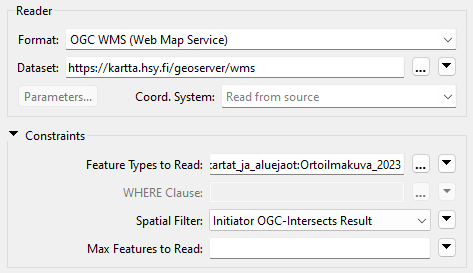
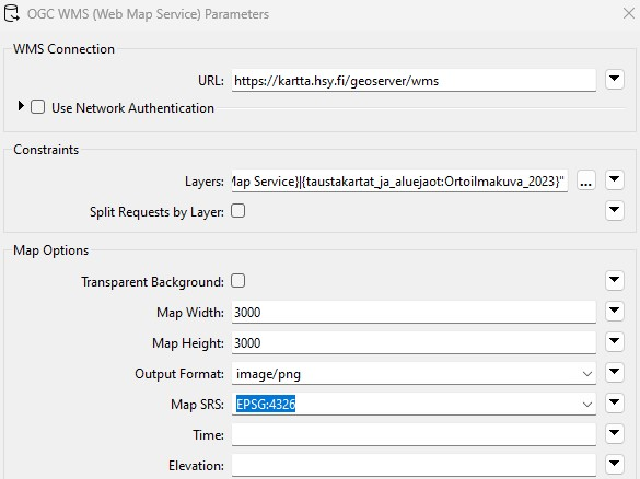
- Read through HSY open data orthoimages WMS
- Merge and clip both images
Implement filtering within the database to streamline the process of reading accessibility data

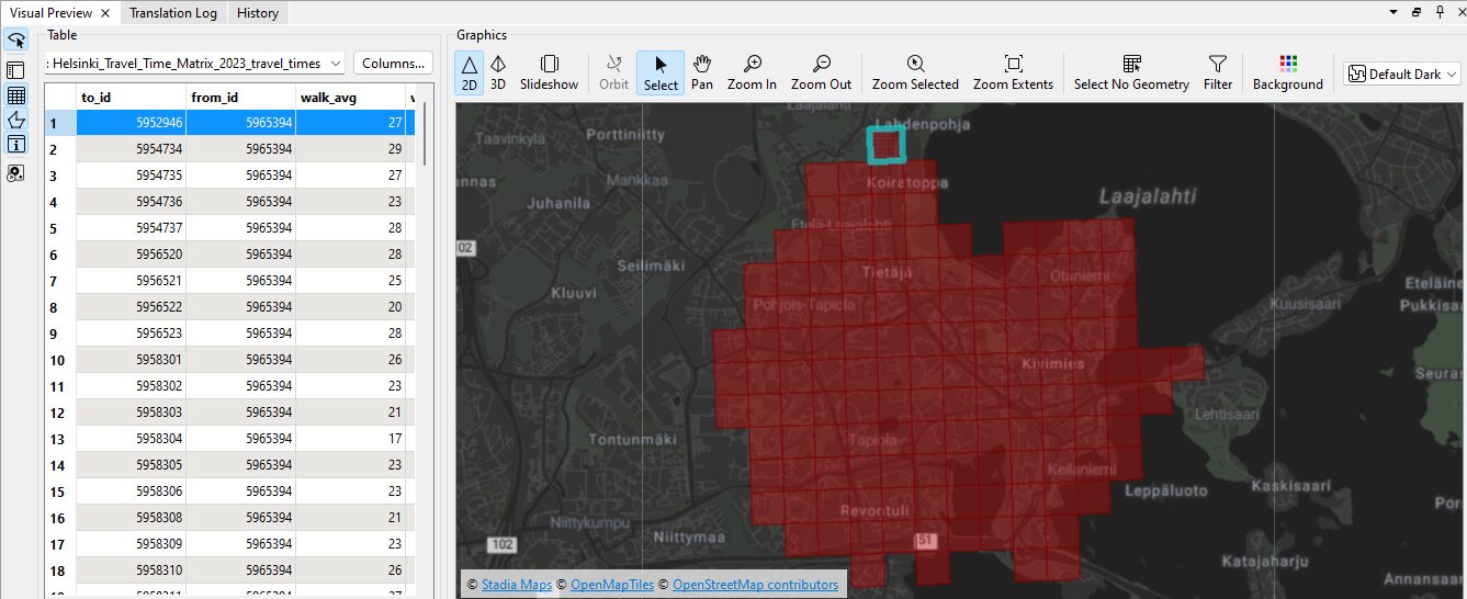
The accessibility data is stored in matrices. For each cell, you have access for all the metrics, time and distance, for this cell on the whole metropolitan area. As the cells are 250m*250m, you can imagine the amount of points/cells. We will use SpatiaLite/GeoPackage indexing to selectively read tiles of interest, optimizing efficiency.
- Initiate the workspace and create a point using the Creator tool.
- Utilize the FeatureReader tool to identify the tile number intersecting our point of interest.
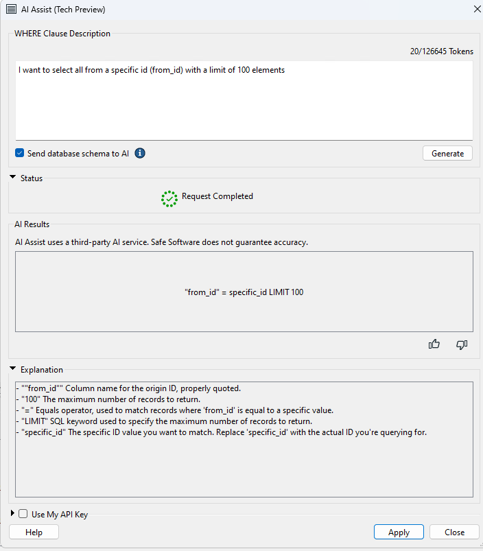
- Further employ the FeatureReader tool to extract relevant information from cells within the identified tile. For users unfamiliar with SQL, FME 2024 offers an AI assistant to facilitate this process. Additionally, the tool allows for the seamless integration of table schema at this stage, enhancing ease of use and flexibility.
Notes:
- This dataset is really rich. Explore the dataset beyond this tutorial to create custom pipelines and deepen your understanding as step by step is tutorial are only here to give a direction and practical example. Experimentation is key to get the know-how
- Employ caching mechanisms to verify the correctness of data at each step of the process, thereby minimizing errors and improving overall efficiency.
Rasterizing our cells with transparency based on time distance.
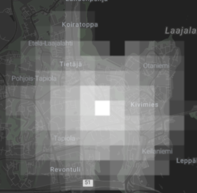
The most commonly used representations for isochrone maps are color gradient and equal time lines. Both can be done with FME but transparency with dark background is great to convey the darkness and cold feeling you get when you walk out during a cold Finnish winter night (or day…).
As we want for the time to reach a point to be reflected as transparency we will compute a ratio based on this time and rasterize our vectors, to help the merging.
-
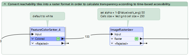
- FeatureColorSetter is necessary to rasterize, we put RGB to 255 to facilitate later merging. We don’t want to use the color from this raster, only its transparency.
- ImageRasterizer tool rasterizes the cells, setting the alpha (transparency) based on the relative time distance from the starting point. As the maximum time is 30 minutes and the time to reach a cell is stored in minutes in “walk_avg” it gives : 1 – (@Value(walk_avg)/30)
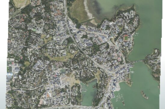
Integrate the orthoimage seamlessly and prepare for merging
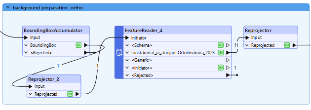
We want to have the orthoimage as background and to prepare to merge it back so with the right level of details and coordinate system.
- BoundingBoxAccumulator allows to select the area of interest.
- Reprojector allows to match the orthoimage coordinate system with the API’s requirements.
- FeatureReader is key for effortless integration with WMS or WMTS. Simply specify the intersection, layer, and image size parameters to proceed with ease.
- Reproject back to the coordinate systems of the original tiles.
I am text block. Click edit button to change this text. Lorem ipsum dolor sit amet, consectetur adipiscing elit. Ut elit tellus, luctus nec ullamcorper mattis, pulvinar dapibus leo.
Merging two rasters together and clip the output
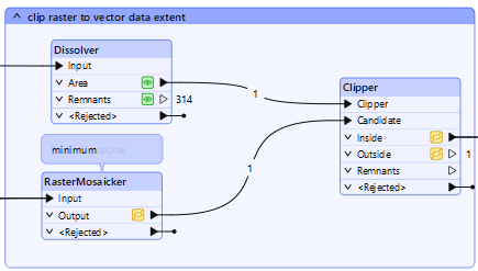
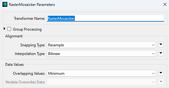
There are different ways to merge rasters in FME but one of the easiest is RasterMosaicker. We will tell about the main points not to forget when using it.
- Push the two rasters into RasterMosaicker in the correct order. The order determines the characteristics of the output image, so verify that the rasters are arranged appropriately. Consider using port order and annotate it to prevent loss of information.
- Set the parameters of RasterMosaicker to utilize the “minimum” value from both images. This ensures that the resulting merged image retains alpha band values from the accessibility cells and colors from the orthoimage.
- Employ Dissolver to refine the output image, ensuring a cohesive result by cutting it with a single polygon.
- Utilize Clipper to clean the output after reprojection, retaining only the relevant portion.

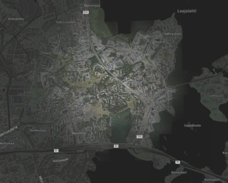
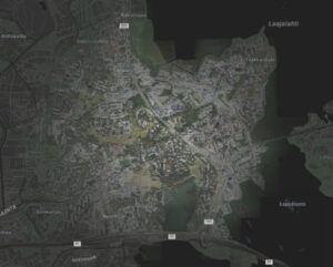
We finally get what we were looking for :
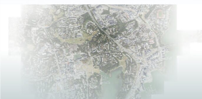
Add a dark background map for a fitting portrayal of the Finnish winter ambiance.
Conclusion
This tutorial has equipped us with the skills to extract data using SQL queries and WFS flux, manipulate raster files with transparency, and leverage FME’s capabilities.
In today’s data-rich landscape, FME emerges as a vital tool for integrating diverse sensor-based data from various open sources. Its ability to swiftly analyze data addresses real-world challenges such as urban planning and recreational route planning in Helsinki. If you’re intrigued by this approach, don’t hesitate to reach out to us for further exploration!

 Suomi
Suomi Svenska