Geospatial imagery and other raster datasets often sit underutilized in archives, rich with potential insights that are hard to extract. Today, a class of AI models called embedding models is changing that. By using embeddings, numerical representations of data that capture its essential patterns, we can unlock information in current and legacy raster data that was previously inaccessible.
In the past, embeddings were mostly an internal step in classification models. For example, a neural network might learn features that help distinguish a cat from a dog, but those features were not typically used directly. In the geospatial domain, you usually still had to train a model on your own labelled data to get usable results.
With generic models like DINOv3, you can now compute embeddings directly on your own imagery, on your own machines. You can still fine-tune them if needed, but as we’ll see, you can already do a lot just by using the pretrained model “as is”. Of course, you can also build on top of them, this is why Meta call it a vision foundation model.
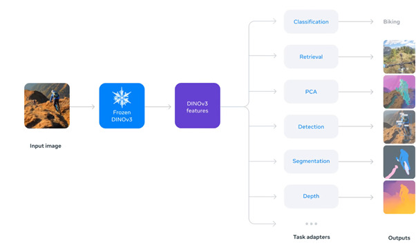
Image from https://ai.meta.com/dinov3/
With the flexibility of Safe Software’s FME (Feature Manipulation Engine) as a low-code integration platform, non-coders can harness these advanced AI capabilities. In this article, we’ll explain embeddings in simple terms and walk through three real use cases where combining an embedding model with FME gives raster datasets a new life. Each scenario is actionable, with data and processes available for readers to experiment with themselves (see the download link at the end).
What Are Embeddings?
In the context of machine learning, embeddings are a way to convert complex data (like an image or text) into a list of numbers (a feature vector) that captures meaningful characteristics of that data. You can think of an embedding as a compact summary or fingerprint of the original content.
For images, an embedding might be a vector of a few hundred or a thousand numbers that collectively represent things like shapes, textures and structures in the patch, but not in an explicit human-readable way. The key idea is that similar data will have similar embeddings. If two image patches both contain dense forest, an embedding model will generate vectors for them that are numerically close to each other. The model doesn’t just look at individual pixels, but also at patterns and context.
This technique compresses vast amounts of visual information into a smaller set of features that represent the data’s meaningful semantics. The power of embeddings is that they make it easy for computers to compare and search content. Instead of comparing raw pixel values (which is impractical), we compare the embeddings. This unlocks operations such as:
- searching images by content
- clustering and classifying scenes by similarity
- detecting anomalies
In short, embeddings turn rich, unstructured data (like raster pixels) into a structured form that we can index and analyze efficiently.
As reference, the same concept was used for text in our RAG article.
A New Life for Existing Raster Datasets
How do embedding models breathe new life into rasters?
Consider a large archive of aerial photos or satellite imagery collected over the years. Traditionally, to find something in these images, say all areas with water bodies or dense forest,, you’d have to manually analyze each image or train a model after labelling a lot of them. An embedding model changes the game by unlocking the content inside the images without extra work. By running each raster image (or even each tile or small patch) through the model, we obtain an embedding vector that represents that image’s content. These embeddings can then be used in multiple ways:
- Content-based search : find what you need, fast.
Because similar images have similar embeddings, you can query the archive for images that match a certain example or pattern. For instance, given one image patch showing a lake, find all other patches with similar water textures. This was nearly impossible to do at scale before; embeddings make it feasible to build a “search engine” for imagery. - Clustering and discovery : reveal hidden structure.
By grouping patches by their embedding vectors, you might automatically discover categories in your dataset: urban, forest, water, bare soil, etc. This unsupervised discovery can reveal trends (like expanding built-up areas or deforestation) that give the dataset new relevance. - Enhancing analyses with new features : combine with other data.
Once images are converted to embeddings (or further distilled into categories or scores), you can cross-reference this information with other datasets to get new insights or fond anomalies.
FME + AI: Low-Code Integration for Everyone
You might be thinking: “This sounds complex , do I need to be a programmer or AI specialist to do this?” . Thankfully, no.
This is where FME comes in. FME is a powerful data integration platform known for its flexibility in handling spatial data, and it provides a no-code/low-code interface. You build workflows by connecting graphical components (transformers) rather than writing code. With FME, you can connect to virtually any data source or format, including large rasters, databases, web services, and now even AI models, all without writing a single line of code.
In our case, the embeddings are computed with DINOv3 and stored either as NumPy (.npy) files per tile or in a database table (DuckDB) with a vector column. FME’s strength lies in how you use them, both before and after the embedding step:
- Before:
- Select objects or areas of interest.
- Build patch grids aligned to your rasters.
- Orchestrate tiling and parallel processing for efficient computation.
- After:
- Join embedding results with vector layers or other attributes.
- Apply filters and thresholds, run spatial joins, group by polygons.
- Automate reporting, visualization and publication in FME Flow.
FME is famously format-agnostic and flexible. It has dozens of raster transformers and support for hundreds of data formats, meaning it can read your legacy data (GeoTIFF, JPEG2000, proprietary formats) and write out results in whatever form you need. Its no-code interface lowers the barrier so non-developers can create sophisticated data pipelines in an understandable, reliable way. Want to load embeddings into a spatial database, or compare them against a shapefile of land parcels? It’s a matter of adding the right transformers.
FME essentially acts as the glue that brings data and AI together: it can connect to databases or APIs, handle large volumes, and schedule or automate tasks in FME Flow for production. Providing a simple app or self-service workspace for end-users on top of these workflows is straightforward.
The result is that advanced image analysis isn’t confined to data scientists: planners, analysts, or any GIS professional can leverage it through FME.
Now, let’s look at three concrete use cases that demonstrate how an embedding model + FME workflow delivers value. Each scenario uses an existing raster dataset and combines it with other data in FME to solve a real problem.
Use Case 1 : Find All Solar Panels from One Example
Question
We have city-wide orthophotos and want to map solar panels. There is no labelled training dataset, and we don’t want to build and maintain a supervised model. Can we start from one known panel and find similar ones?
Idea
Because DINOv3 embeddings capture texture and structure, we can:
- Pick one patch that clearly contains solar panels.
- Look for all patches whose embedding is closest to that reference in the 1024-dimensional space.
- Bring those patches back to map coordinates and visualize them.
No supervised training, just similarity search in embedding space.
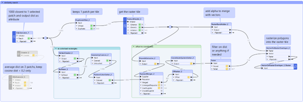
Workflow in FME (conceptually)
-
Rebuild the patch grid
- Use FME to generate a grid aligned with the raster tiling (cells of 8 m × 8 m, the physical size of a 16×16 pixel patch at 0.5 m resolution).
- Each grid cell corresponds to a DINOv3 patch, identified by tile name and patch indices (row, column).
-
Select a reference patch
- Load orthophotos as background in Data Inspector.
- Click on a grid cell that clearly covers solar panels (good orientation, clear panels, limited shadow).
- Extract its tile/row/col and look up its embedding in the DuckDB table.
3. Find similar patches
-
- In a small SQL step (provided in the example), compute the distance between the reference embedding and all other embeddings (e.g. cosine or Euclidean distance).
- Sort patches by distance and keep, for example, the 1000 closest as a first pass.
- Optionally, apply a distance threshold (e.g. keep only patches with distance below a tuned value)
4. Back to the map
-
-
- Join the selected embeddings back to their patch grid features in FME.
- Turn each patch into a rectangle in real-world coordinates (using tile bounds and patch indices).
- Color patches by distance to the reference (closer = more likely solar panel).
-
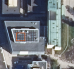
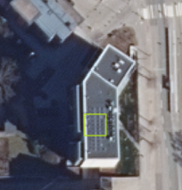
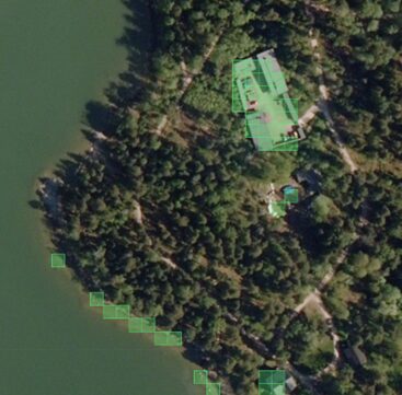
What you see
In Data Inspector you see:
- The orthophoto in the background
- A grid of patches
- Highlighted patches that DINOv3 considers similar to the example solar panel
You’ll notice:
- Many true positives (solar panel arrays on roofs)
- Some false positives (dark roof elements, skylights, some industrial rooftops)
You can refine the results by:
- Setting a stricter distance threshold
- Using multiple reference patches (different panel sizes, orientations, rooftop types) and combining results
- Restricting to areas with buildings using a vector building footprint layer
The end result is a solar panel candidate layer generated with very little manual effort.
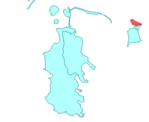
Use Case 2 : Where Did the City Change Between 2014 and 2020?
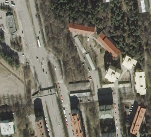
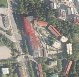
Situation in 2014 vs 2020 (with changed patches in red)
Question
We have orthophotos for 2014 and 2020 at the same resolution and coverage. We’d like to see:
- Where new buildings appeared
- Where large land cover changes happened
- Without manually comparing the two mosaics, patch by patch
Idea
For each patch location (same tile, same row/col), we compare:
- The embedding in 2014
- The embedding in 2020
If a location didn’t change much (same buildings, similar vegetation), the embeddings will be close. If it changed a lot (new construction, major clearing), the embeddings will be far apart.
So we define a change score:
change = distance(embedding_2014, embedding_2020) and use FME to map and filter on that score.
Workflow in FME
-
Run DINOv3 on both years
- Use identical tiling (same grid, same patch indices) for 2014 and 2020.
- For each tile + patch index we now have two embeddings: one from 2014, one from 2020.
-
Compute change per patch
- In DuckDB, compute the distance between the 2014 and 2020 embeddings for each patch.
- Store this value as in the table (“delta_2014”).
-
Select changed patches
- In FME, read the table and apply a first filter like delta_2014> 0.25 to remove very small changes and noise.
- Then use a Tester transformer to keep only strong changes, e.g. delta_2014> 0.80.
- These threshold values are chosen empirically by looking at the distribution of distances and visually inspecting results; they can be tuned for each dataset.
-
Visualize as polygons or raster
Two options:
-
- Polygons: represent each patch as a rectangle and overlay them on the 2020 orthophoto. Darker color = bigger change score.
- Change raster: use ImageRasterizer to convert changed patches into a raster layer, give it a semi-transparent color, and blend it with the 2020 imagery using RasterMosaicker.
What you see
Typical patterns that pop out include:
- New residential areas at the edge of the city
- New roads or widened road corridors
- Industrial developments and large clearings
Interestingly, some natural changes (like seasonal vegetation variation) may still have relatively low distances if the overall texture remains similar. This is useful: the method tends to highlight structural changes more than small spectral differences.
This workflow becomes a reusable change-detection tool. When new imagery arrives, you run the same pipeline and immediately see where the most significant changes are.
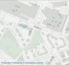
Use Case 3 : Are My Vegetation / Zoning Polygons Consistent with the Imagery?
Question
The City of Helsinki provides various zoning and land-use layers. Suppose we take a vegetation or green area polygon layer. It is meant to represent parks, green corridors, and similar spaces.
We want to know:
- Are there parts of these polygons that visually look very different from the rest?
- Did some areas get paved or built over but never updated in the vector data?
- Are there “holes” (roads, parking lots, buildings) inside zones which are still classified as green?
Idea
Inside a given polygon, most patches should look broadly similar (trees, grass, paths). We can:
- Collect embeddings of all patches inside each polygon.
- Compute the median embedding for that polygon (a kind of “typical” patch for that area).
- Measure how far each patch is from this median embedding.
- Flag patches that are much farther than the typical distance.
Those patches are outliers inside the polygon, they might indicate misclassification, new construction, or simply interesting anomalies.
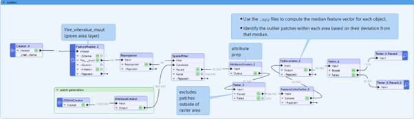
Workflow in FME
-
Intersect polygons with patch grid
- Use FME to generate the same patch grid as before (8 m × 8 m cells).
- Intersect this grid with the vegetation polygons.
- Keep only patches that fall inside each polygon and carry over the polygon ID.
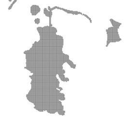
Green area objects as polygons and as a grid
- 1. Load embeddings for these patches
- Using the tile/row/col attributes, look up the corresponding embeddings from the .npy files.
- A PythonCaller reads embeddings and attaches them to each patch feature.
- 2. Compute per-polygon median and outliers
Inside PythonCaller (or an external script triggered from FME):
-
- Group patches by polygon ID.
- For each group, stack all embeddings into an array.
- Compute the median embedding of that group.
- Compute distance from each patch’s embedding to this median.
- Determine a threshold based on the distribution (for example, mark the top 5% farthest patches as outliers).
- Return two attributes to FME:
- dist_to_median
- is_outlier (0/1)
-
3. Inspect and act
- Use a Tester in FME to filter to is_outlier = 1.
- Visualize those patches over the orthophoto and the polygon boundaries in Data Inspector.
What you see?
The outlier patches often correspond to:
- Buildings encroaching into green areas
- Parking lots, roads, or construction sites inside polygons still classified as vegetation
- Bare soil or water patches that don’t match the majority of the polygon
This gives you a quality-control tool for vector layers driven directly by the imagery underneath. You don’t label anything; you simply use the inherent structure of the embeddings.
Why Combining FME and DinoV3 Works So Well?
Across all three use cases, the pattern is the same:
- DINOv3 provides a general, reusable representation of every image patch.
- We don’t train new models; we reuse these embeddings for different questions.
- FME provides the data plumbing, spatial logic and user-friendly UI to:
- connect embeddings to tiles, rasters and vector data
- perform selections, aggregations and QA
- produce outputs that decision-makers can understand (maps, layers, tables)
This gives existing orthophoto archives a second life:
- as a searchable database of content (similarity search)
- as a change detector over time (embedding differences)
- as a consistency checker for other spatial layers (outliers inside polygons)
Because everything is built in FME, non-coders can run, adapt and extend these workflows without becoming ML engineers.
Ready to Try It Yourself?
These techniques are not just theoretical, you can start experimenting with your own data, or try out our examples.
As the set up requires a bit of data and also to install something similar to micromamba and some SQL pre-processing, we could not just publish to FME hub. We’ve prepared a sample template containing the FME workspace with cached data for the three use cases described above, you can download it with the link below or contact us to get more information.
Load the workspace in FME, follow the embedded annotations, and you’ll be able to reproduce the results or tweak the workflows for your own needs.
By embracing modern embedding models and the power of FME’s low-code platform, you can extract new insights from old raster datasets with ease. What will you discover in your imagery?

 Suomi
Suomi English